
Amdahl's Law and Speedup
Last updated on 2026-08-27 | Edit this page
Overview
Questions
- What factors limit how much parallelism can help?
- How do I predict maximum speedup?
- How do I measure if parallelism is working?
Objectives
- Understand Amdahl’s Law and its implications
- Calculate theoretical speedup for different serial fractions
- Recognize when parallelization is not worth the effort
Amdahl’s Law: The Reality Check
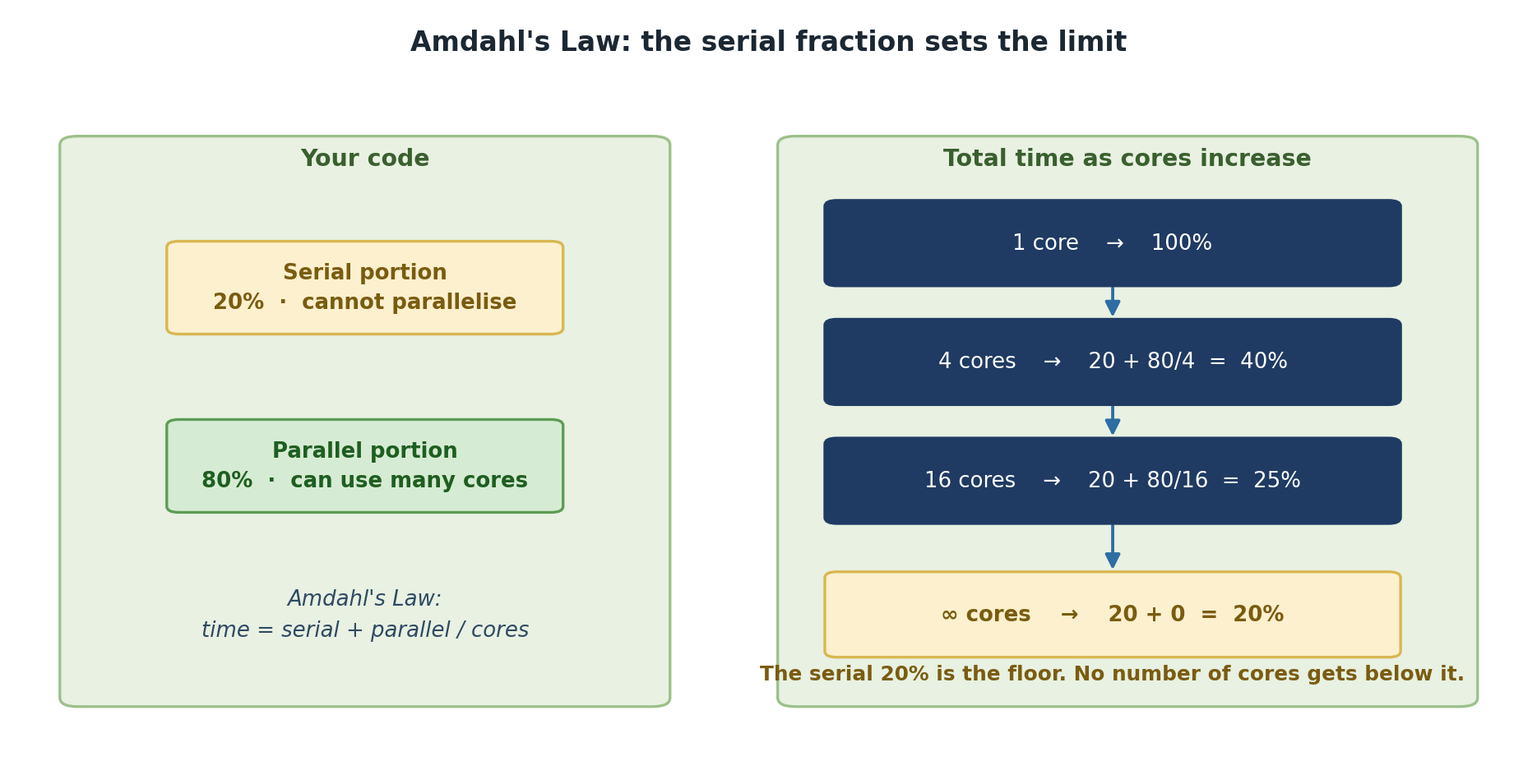
Not all code can be parallelized. Some parts are inherently serial: reading input files, initializing data structures, writing output, sequential dependencies.
Amdahl’s Law quantifies maximum speedup:
\[S_p = \frac{1}{f_s + (1-f_s)/p}\]
Where \(f_s\) = serial fraction and \(p\) = number of processors.
Amdahl’s Law in Action
10% serial, 90% parallel with 16 processors:
\[S_{16} = \frac{1}{0.1 + 0.9/16} = \frac{1}{0.156} = 6.4\]
Even with 16 processors, only 6.4x speedup. The serial portion is the bottleneck.
5% serial → \(S_{16} = 9.2\). 1% serial → \(S_{16} = 13.9\).
Key Insight
The serial fraction is your enemy. Even a small serial portion becomes a huge bottleneck at scale. This means:
- Measure before parallelizing: Profile your code to find bottlenecks
- Don’t parallelize prematurely: Make sure the parallel portion is actually the bottleneck
- Choose the right granularity: Balance communication overhead against computation
Challenge
Calculating Amdahl’s Law
For each scenario, calculate the theoretical speedup on 8 processors:
Scenario 1: 99% parallelizable. \(S_8 = \frac{1}{0.01 + 0.99/8} = ?\)
Scenario 2: 95% parallelizable. \(S_8 = \frac{1}{0.05 + 0.95/8} = ?\)
Scenario 3: 80% parallelizable. \(S_8 = \frac{1}{0.20 + 0.80/8} = ?\)
Scenario 1: \(S_8 = 1/0.1338 = 7.48\) (93.5% efficiency)
Scenario 2: \(S_8 = 1/0.1688 = 5.92\) (74% efficiency)
Scenario 3: \(S_8 = 1/0.30 = 3.33\) (42% efficiency – may not be worth it!)
Measuring in Practice
BASH
# Create a test program
cat > test_serial.py << 'PYTHON'
import time

# Serial initialization (10% of runtime)
print("Initializing...")
time.sleep(1)

# Parallelizable work (90% of runtime)
start = time.time()
result = 0
for i in range(100000000):
    result += i
elapsed = time.time() - start
print(f"Elapsed: {elapsed:.2f} seconds")
PYTHON

python3 test_serial.py
Questions to consider: 1. How long did initialization take relative to computation? 2. What does Amdahl’s Law predict with 4 cores? 3. Could you optimize the serial portion instead?
- Amdahl’s Law shows that serial code limits maximum speedup
- Even small serial fractions (5-10%) become significant bottlenecks at scale
- Profile serial code first to identify the true bottleneck
- Don’t parallelize prematurely; ensure the payoff justifies the complexity